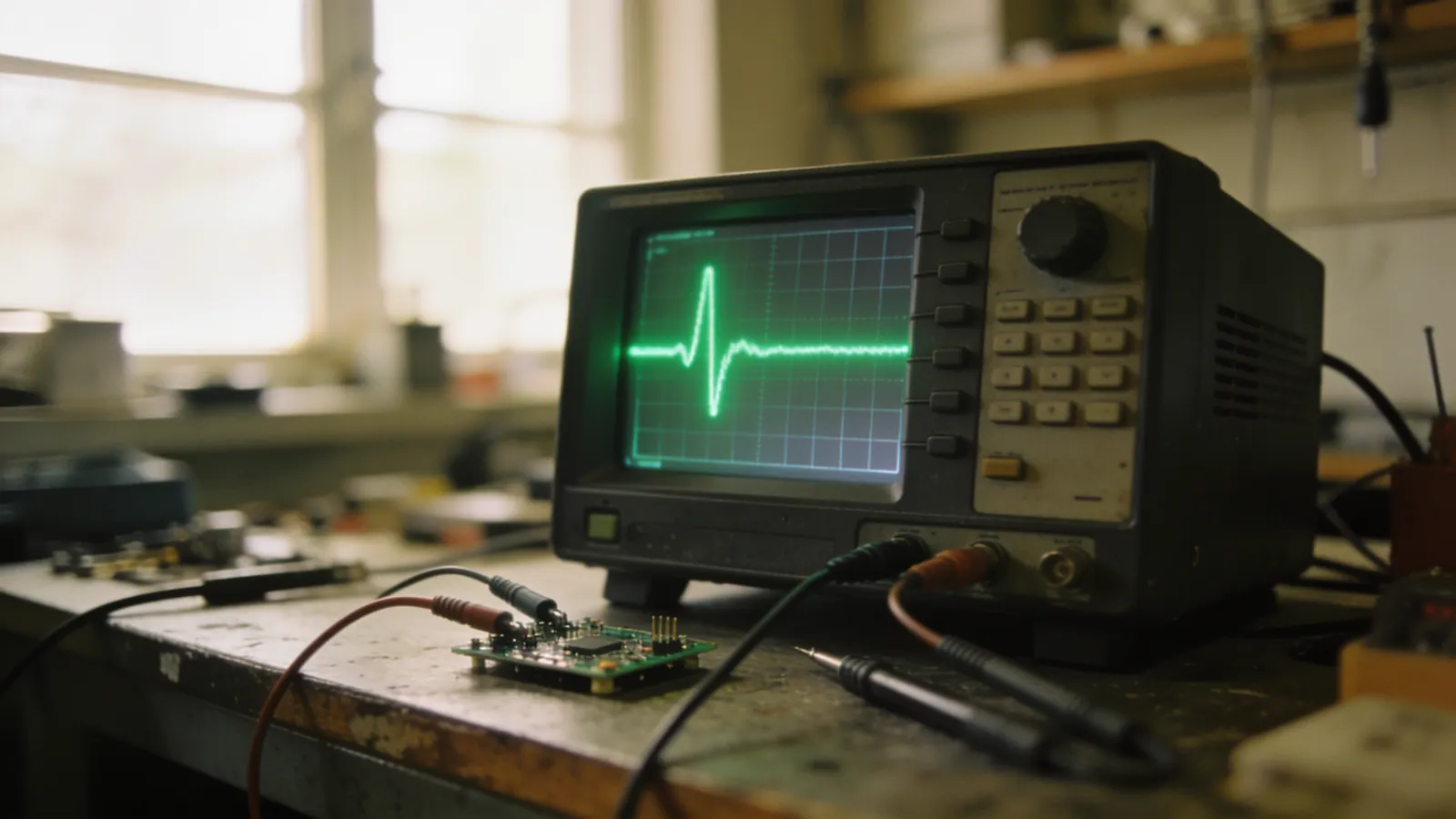
PID control is one of the most widely used—and most misunderstood—algorithms in engineering. Although its name may seem complicated, what it does is extremely intuitive: keeping something where it’s supposed to be.
Whether an air conditioner is keeping a room at 22 degrees, a drone is hovering in the air, or a line-following robot is moving along a track, the same three terms are always at work. In this article, I’ll explain PID using intuition rather than formulas, and then we’ll turn it into an application that runs on an Arduino.
The basic idea: error
Every control system starts with a single number: the error.
hata = hedef_deger - olculen_degerIf the robot is 2 cm to the right of the line, the error is 2. If the motor’s speed should be 100 rpm but is actually 80 rpm, the error is 20. PID’s sole task is to reduce this number to zero.
But is knowing the error enough? No. Because the answer to the question “How much correction should I make?” doesn’t depend solely on the magnitude of the error.
P — Proportional term
The most intuitive component: if the error is large, correct it significantly; if it’s small, correct it slightly.
P = Kp * hataIt’s similar to turning the steering wheel. If you’ve veered far off course, you turn the wheel a lot; if you’ve veered only a little, you turn it slightly.
In the simulator below, you can adjust all three coefficients in real time. To start, set Ki and Kd to zero and experiment only with Kp: at small values, the system moves slowly toward the target; as you increase the value, it speeds up; and past a certain point, it begins to oscillate around the target. Seeing these three behaviors with your own eyes teaches you more than pages of explanation ever could.
Two Problems with P
1. Steady-state error. As the error decreases, the correction also decreases. Eventually, the correction becomes too small to overcome friction, and the system never reaches the target—it always remains slightly below it.
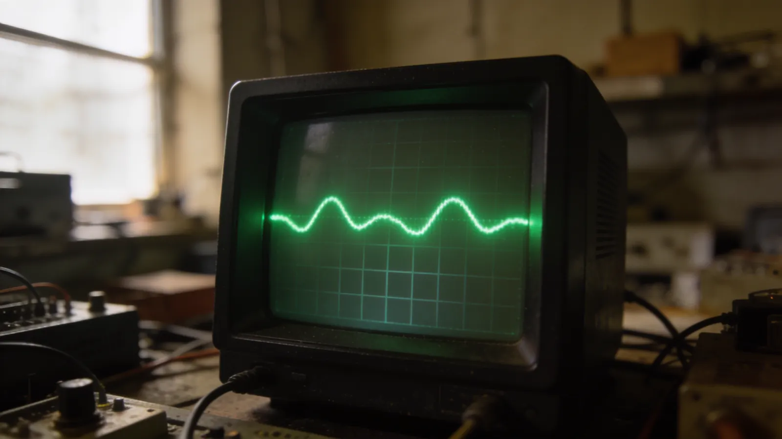
2. Oscillation. If you increase Kp, the steady-state error decreases, but the system overshoots the target, swings back, and overshoots again. It’s like pushing a heavy door quickly and being unable to stop it.
I — Integral Term
The integral looks at the total error over time. It carries the information that “I’ve been below the target for a long time.”
integral = integral + hata;
I = Ki * integral;
A small but persistent error continuously increases the integral; the growing integral forces the output, and eventually, the friction is overcome. This is what resolves the persistent error that P cannot resolve.
Integral buildup (windup)
The I term is dangerous. If the system cannot reach the target (the motor is already at full power, or there is an obstacle), the integral continues to grow. When the obstacle is removed, the accumulated massive integral sends the system far beyond the target.
There are two standard solutions:
// 1) Integrali sınırla
integral = constrain(integral, -MAKS_INTEGRAL, MAKS_INTEGRAL);

// 2) Çıkış doyuma ulaştıysa integrali biriktirme
if (cikis < MAKS_CIKIS && cikis > MIN_CIKIS) {
  integral += hata;
}In robotics projects, the I term is often unnecessary, even harmful. In a line-following robot, Ki=0 usually yields the best results. Add the I term only if there is a constant disturbing force (gravity, continuous friction, constant wind).
D — Derivative term
The derivative looks at how fast the error is changing. It predicts the future.
turev = hata - onceki_hata;
D = Kd * turev;
If the error is decreasing rapidly, it means the system is approaching the target quickly—the D term acts as a brake and prevents overshoot. That’s why D is also called “damping.”
Derivative noise
The weak point of the D term is noise. A small spike in the measurement creates a large spike in the derivative. Using a high Kd with a noisy analog sensor causes motors to vibrate.
Two solutions:
// 1) Türeve alçak geçiren filtre uygula
turev_filtreli = 0.7 * turev_filtreli + 0.3 * (hata - onceki_hata);

// 2) Hata yerine ölçümün türevini al (türev vuruşunu önler)
turev = -(olcum - onceki_olcum);
The second method also prevents the output from spiking (derivative kick) when the target value changes suddenly.
Combining the three
float Kp = 2.0, Ki = 0.0, Kd = 12.0;

float integral    = 0;
float oncekiHata  = 0;
unsigned long sonZaman = 0;
const unsigned long PERIYOT = 10;   // ms — SABİT tutun

void loop() {
  if (millis() - sonZaman < PERIYOT) return;
  sonZaman = millis();

  float olcum = sensorOku();
  float hata  = HEDEF - olcum;

  float turev = hata - oncekiHata;
  oncekiHata  = hata;

  float cikis = Kp * hata + Ki * integral + Kd * turev;
  cikis = constrain(cikis, -255, 255);

  // Anti-windup: sadece doyumda değilken biriktir
  if (cikis > -255 && cikis < 255) {
    integral += hata;
    integral = constrain(integral, -1000, 1000);
  }

  cikisUygula(cikis);
}
The most critical line here PERIYOT control. PID mathematics assumes a fixed sampling interval. If the cycle sometimes lasts 5 ms and sometimes 50 ms, the I and D terms become meaningless.
Tuning the coefficients: a systematic method
Instead of trying random numbers, follow this sequence. Change a single coefficient at each step and record the result.
| Step | Action | Expected behavior |
|---|---|---|
| 1 | Ki=0, Kd=0. Start Kp with a small value. | The system gradually approaches the target but does not quite reach it. |
| 2 | Increase Kp by doubling it. | The response speeds up, and eventually oscillation begins. |
| 3 | Pull back 40–60% from the oscillation point. | A fast but controlled reaction. |
| 4 | Add Kd, starting at 5 times the value of Kp. | Oscillation begins to die down, and overshoot decreases. |
| 5 | Increase Kd; if oscillation begins, reduce it. | Soft and quick settling. |
| 6 | If there is a persistent error, add a very small Ki. | The error will slowly decrease to zero. |
Diagnosis based on symptoms
| What you see | Possible cause | Try |
|---|---|---|
| Very slow response | Kp is low | Increase Kp |
| Oscillation around the setpoint | Kp is high, Kd is low | Increase Kd or decrease Kp |
| High-frequency oscillation | Kd is too high / noise | Decrease Kd, filter the measurement |
| Cannot reach the target at all | Persistent error, no I | Add a small Ki |
| Large overflow followed by recovery | Integral bloat | Limit the integral |
| Irregular, unpredictable | Variable cycle period | Set a fixed period |
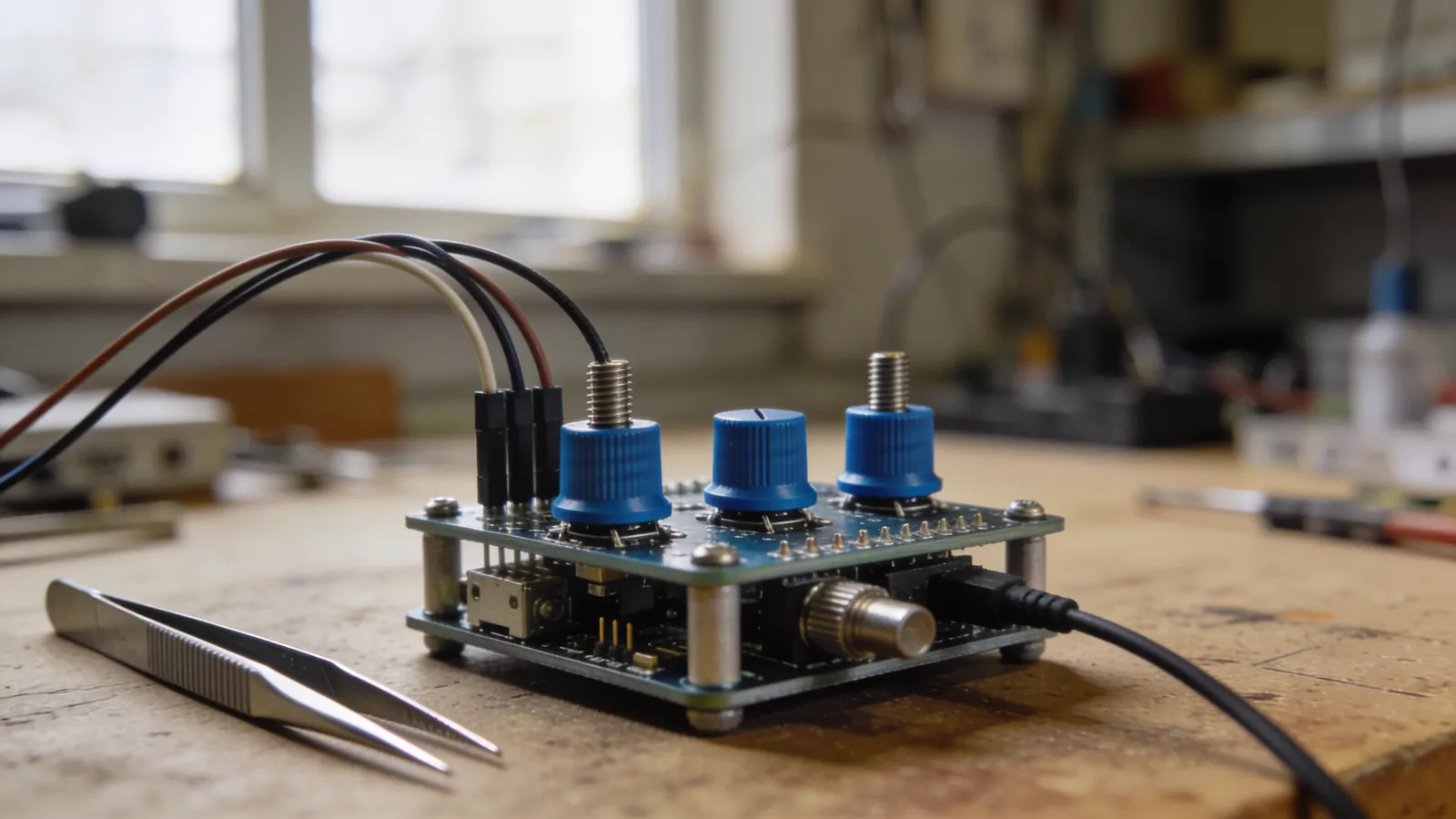
Being able to change the coefficients in real time reduces the setup time from hours to minutes. Connect three potentiometers, or if you’re using an ESP32, send the coefficients via Bluetooth. Trying to make adjustments by uploading code every time is the biggest waste of time.
Three real-world applications
1. Line-following robot
Target: the center of the line-following robot. Measurement: position from the sensor array. Output: the difference in speed between the left and right motors.
int hata = konumHesapla() - MERKEZ;
int duzeltme = Kp * hata + Kd * (hata - oncekiHata);
motorSur(TABAN + duzeltme, TABAN - duzeltme);
Typical values: Kp = 0.05–0.3, Ki = 0, Kd = 0.5–3. See the line-following robot guide for details.
2. Motor Speed Control
Target: constant RPM. Measurement: RPM calculated from the encoder. Output: PWM value.
The I term is required here because friction and load are constant disturbing forces. I explained the use of encoders in the motor selection guide.
3. Wall-following
Goal: Constant distance from the wall. Measurement: Side-mounted distance sensor. Output: Turn angle.
Sensor selection is critical in this application: wide-angle ultrasonic sensors can be unreliable at corners, while narrow-beam ToF sensors are more stable. See the distance sensors guide for a comparison.
Making the PID Reusable
Instead of copying and pasting the same PID code into every project, write a small class. Write it once, use it everywhere—and when you fix a bug, it’s fixed in every project.
class PID {
  public:
    PID(float kp, float ki, float kd, float cikisSiniri = 255)
      : _kp(kp), _ki(ki), _kd(kd), _sinir(cikisSiniri) {}

    void ayarla(float kp, float ki, float kd) { _kp = kp; _ki = ki; _kd = kd; }

    void sifirla() { _integral = 0; _oncekiOlcum = 0; _ilk = true; }

    float hesapla(float hedef, float olcum, float dt) {
      float hata = hedef - olcum;

      // Türevi ölçümden al: hedef değişince çıkış sıçramaz
      float turev = _ilk ? 0 : -(olcum - _oncekiOlcum) / dt;
      _oncekiOlcum = olcum;
      _ilk = false;

      float cikis = _kp * hata + _ki * _integral + _kd * turev;

      // Anti-windup: sadece doyumda değilken biriktir
      if (cikis < _sinir && cikis > -_sinir) {
        _integral += hata * dt;
      }

      return constrain(cikis, -_sinir, _sinir);
    }

  private:
    float _kp, _ki, _kd, _sinir;
    float _integral = 0, _oncekiOlcum = 0;
    bool  _ilk = true;
};
Usage:
PID cizgiPid(0.08, 0.0, 1.2, 255);

void loop() {
  static unsigned long son = 0;
  unsigned long simdi = millis();
  if (simdi - son < 10) return;
  float dt = (simdi - son) / 1000.0;
  son = simdi;

  float duzeltme = cizgiPid.hesapla(MERKEZ, konumHesapla(), dt);
  motorSur(TABAN + duzeltme, TABAN - duzeltme);
}
Two details here are important. First, dtcalculating it based on the actual elapsed time; this way, even if the cycle period shifts slightly, the I and D terms remain accurate. Second, sifirla() the function: if you don’t clear the accumulated integral when the robot stops and restarts, the first movement will start with a jump.
Feedforward: The Missing Half of PID
PID is reactive—it does nothing until an error occurs. However, you may already know about certain disturbances in advance. Feedforward adds this known component directly to the output.
A simple example: motor speed control. You roughly know the PWM value required for a specific speed. If you add this to the PID’s correction, the PID deals only with the remaining difference:
// Sıfırdan başlamak yerine doğru değere yakın başla
float ileriBesleme = hedefHiz * PWM_PER_RPM;
float duzeltme     = hizPid.hesapla(hedefHiz, olculenHiz, dt);
float cikis        = ileriBesleme + duzeltme;
PWM_PER_RPM To find the coefficient, simply measure the motor’s RPM at a few PWM values and establish a direct proportional relationship.
Result: The system reaches the target much faster, and the PID coefficients can be smaller—and therefore more stable. In systems operating against gravity, such as a robotic arm, feedforward is almost mandatory.
When Not to Use PID
PID isn’t the solution to every problem:
- If on/off control is sufficient (heater, fan), PID introduces unnecessary complexity. A simple thermostat logic with hysteresis is more appropriate.
- If the system has significant delay (large thermal mass), PID struggles; feedforward must be added.
- If the system is nonlinear, a single set of coefficients will not yield good results at every operating point. Gain scheduling may be required.
Summary
- P looks at the current error → the main driving force.
- I looks at the past error → closes out the steady-state error; use with caution.
- D predicts the future → dampens oscillations, sensitive to noise.
Once you learn how to properly set up a PID loop, you can use the same tool across a wide range of applications, from robotics to temperature control, and from drone stabilization to CNC axis control. That’s why it’s worth taking the time to learn.
Frequently asked questions
PID kontrol nedir, ne işe yarar?
PID, ölçülen bir değeri istenen hedefte tutmaya yarayan bir kontrol algoritmasıdır. Hedefle gerçek değer arasındaki farkı (hata) üç açıdan değerlendirir: P hatanın büyüklüğüne, I hatanın zaman içindeki birikimine, D hatanın değişim hızına bakar. Üçünün toplamı düzeltme sinyalini oluşturur.
PID katsayıları nasıl bulunur?
En pratik yöntem elle ayardır: Ki ve Kd sıfırken Kp’yi sistem sürekli salınıma girene kadar artırın, sonra %40–60 geri çekin. Ardından Kd’yi salınım sönene kadar yükseltin. Ki’yi en son ve çok küçük adımlarla, sadece kalıcı hata varsa ekleyin.
Sadece P kontrol yeterli mi?
Birçok robot uygulamasında evet. Çizgi izleyen robotlar düşük hızda saf P ile gayet iyi çalışır. D bileşeni hız arttıkça, I bileşeni ise yerçekimi veya sürtünme gibi sabit bir bozucu kuvvet varsa gerekli hale gelir.
Integral şişmesi (windup) nedir?
Sistem hedefe ulaşamazken integral teriminin sürekli büyümesidir. Hata sonunda kapansa bile birikmiş integral çıkışı zorlamaya devam eder ve sistem hedefi büyük bir taşmayla aşar. Çözüm, integral terimini constrain() ile sınırlamak veya çıkış doyuma ulaştığında integrali dondurmaktır.
PID döngüsü ne sıklıkla çalışmalı?
Döngü periyodu sabit olmalı ve sistemin tepki süresinden en az 10 kat hızlı olmalı. Çizgi izleyen robotlar için 100–1000 Hz, sıcaklık kontrolü için 1–10 Hz uygundur. Değişken periyot, D teriminde büyük gürültü üretir.
Comments
0No comments yet. Be the first to comment!